Promotion
Use code SIZZLE26 for 25% off sitewide!
By clicking “Accept,” you agree to the use of cookies and similar technologies on your device as set forth in our Cookie Policy and our Privacy Policy. Please note that certain cookies are essential for this website to function properly and do not require user consent to be deployed.
The Theoretical Minimum
What You Need to Know to Start Doing Physics

Contributors
Formats and Prices
- On Sale
- Apr 22, 2014
- Page Count
- 256 pages
- Publisher
- Basic Books
- ISBN-13
- 9780465038923
Price
$12.99Price
$16.99 CADFormat
Format:
- ebook $12.99 $16.99 CAD
- Trade Paperback $18.99 $24.99 CAD
This item is a preorder. Your payment method will be charged immediately, and the product is expected to ship on or around April 22, 2014. This date is subject to change due to shipping delays beyond our control.
Buy from Other Retailers:
A New York Times Bestseller
A Wall Street Journal Best Book of the Year
“Beautifully clear explanations of famously ‘difficult’ things.” ―Wall Street Journal
If you ever regretted not taking physics in college – or simply want to know how to think like a physicist – this is the book for you. In this bestselling introduction to classical mechanics, physicist Leonard Susskind and hacker-scientist George Hrabovsky offer a first course in physics and associated math for the ardent amateur. Challenging, lucid, and concise, The Theoretical Minimum provides a tool kit for amateur scientists to learn physics at their own pace.
Series:
-
“Beautifully clear explanations of famously ‘difficult things.’”Wall Street Journal
-
“A spectacular effort to make the real stuff of theoretical physics accessible to amateurs.”Science News
-
“Very readable. Abstract concepts are well explained.... [The Theoretical Minimum] does provide a clear description of advanced classical physics concepts, and gives readers who want a challenge the opportunity to exercise their brain in new ways.”Physics World
-
“Readers ready to embrace their inner applied mathematics will enjoy this brisk, bare-bares introduction to classical mechanics.”Publishers Weekly
-
“Every minute of our lives is now dependent on technology, yet the wonders of basic science are foreign to many of us. Everyone who remembers even a bit of math should read this inviting and accessible account of ‘what you need to know to start doing physics.’”Wall Street Journal, “Best Book of the Year”
-
“What a wonderful and unique resource. For anyone who is determined to learn physics for real, looking beyond conventional popularizations, this is the ideal place to start.”Sean Carroll, New York Times-bestselling author of The Biggest Ideas in the Universe